Margins for Continuous Variable Interacted With Discrete
The margins command can be a very useful tool in understanding and interpreting interactions. We will illustrate the command in two examples using the hsbdemo dataset.
use https://stats.idre.ucla.edu/stat/data/hsbdemo, clear
Example 1
We will begin with a model that has a categorical by categorical interaction (female by prog) along with a categorical by continuous interaction (honors by read). To keep things somewhat simple, the two interactions have no terms in common. We will begin by running the following regression model.
regress write female##prog honors##c.read Source | SS df MS Number of obs = 200 -------------+------------------------------ F( 8, 191) = 44.21 Model | 11609.4878 8 1451.18597 Prob > F = 0.0000 Residual | 6269.38724 191 32.824017 R-squared = 0.6493 -------------+------------------------------ Adj R-squared = 0.6347 Total | 17878.875 199 89.843593 Root MSE = 5.7292 ------------------------------------------------------------------------------ write | Coef. Std. Err. t P>|t| [95% Conf. Interval] -------------+---------------------------------------------------------------- 1.female | 4.777377 1.751007 2.73 0.007 1.323584 8.231171 | prog | 2 | 2.284045 1.520393 1.50 0.135 -.7148712 5.282962 3 | -4.190142 1.769368 -2.37 0.019 -7.680154 -.7001312 | female#prog | 1 2 | -2.493487 2.071853 -1.20 0.230 -6.580138 1.593164 1 3 | 2.339986 2.387059 0.98 0.328 -2.368397 7.048369 | 1.honors | 28.17233 6.543047 4.31 0.000 15.26641 41.07824 read | .369414 .0553672 6.67 0.000 .2602043 .4786236 | honors#| c.read | 1 | -.3200391 .1112185 -2.88 0.004 -.5394134 -.1006648 | _cons | 28.80342 3.131345 9.20 0.000 22.62696 34.97988 ------------------------------------------------------------------------------
As you can see the honor#c.read interaction is significant along with all the other one degree of freedom tests. There are two multi-degree of freedom tests that we need to follow up on using the testparm command.
testparm female#prog ( 1) 1.female#2.prog = 0 ( 2) 1.female#3.prog = 0 F( 2, 191) = 3.06 Prob > F = 0.0493 testparm i.prog ( 1) 2.prog = 0 ( 2) 3.prog = 0 F( 2, 191) = 8.81 Prob > F = 0.0002
The female#prog interaction is significant along with the two degree of freedom test for prog. Some people might call this the main effect for prog but that is not correct. Since we are using indicator (dummy) coding, the test for prog is really testing the effect of prog when female equals zero, that is, among males. This can also be replicated using the commands:
contrast prog@female Margins : asbalanced ------------------------------------------------ | df F P>F -------------+---------------------------------- prog@female | male | 2 8.81 0.0002 female | 2 0.87 0.4186 Joint | 4 4.73 0.0012 | Denominator | 191 ------------------------------------------------ contrast prog@0.female Margins : asbalanced ------------------------------------------------ | df F P>F -------------+---------------------------------- prog@female | male | 2 8.81 0.0002 | Denominator | 191 ------------------------------------------------
If we multiply the F-ratio for prog by the numerator degrees of freedom, we get a value scaled like a chi-square. Thus, 2*r(F) = 17.616468 which is a value we will see again in a little while.
We can run the same model using the anova command. The anova will appear to be somewhat different because the model is parameterized differently but it is the exact same model.
anova write female##prog honors##c.read Number of obs = 200 R-squared = 0.6493 Root MSE = 5.72922 Adj R-squared = 0.6347 Source | Partial SS df MS F Prob > F ------------+---------------------------------------------------- Model | 11609.4878 8 1451.18597 44.21 0.0000 | female | 922.674277 1 922.674277 28.11 0.0000 prog | 465.899583 2 232.949791 7.10 0.0011 female#prog | 200.694275 2 100.347137 3.06 0.0493 honors | 608.523046 1 608.523046 18.54 0.0000 read | 424.568626 1 424.568626 12.93 0.0004 honors#read | 271.796348 1 271.796348 8.28 0.0045 | Residual | 6269.38724 191 32.824017 ------------+---------------------------------------------------- Total | 17878.875 199 89.843593
Note that the F-ratio for female#prog is the same as that from the testparm command and that the F-ratio for honors#read is the same as the t-value squared from the regression output ((-.3200391/.1112185)^2 = (-2.8775707)^2 = 8.2804133).
Next, we will use estimates store to save this model before using margins with the post option.
estimates store m1
We are finally ready to use the margins command to look at the female#prog interaction.
margins female#prog, asbalanced post Predictive margins Number of obs = 200 Expression : Linear prediction, predict() at : female (asbalanced) prog (asbalanced) honors (asbalanced) ------------------------------------------------------------------------------ | Delta-method | Margin Std. Err. z P>|z| [95% Conf. Interval] -------------+---------------------------------------------------------------- female#prog | 0 1 | 53.82626 1.37582 39.12 0.000 51.1297 56.52281 0 2 | 56.1103 .9608622 58.40 0.000 54.22705 57.99356 0 3 | 49.63611 1.375616 36.08 0.000 46.93996 52.33227 1 1 | 58.60363 1.256171 46.65 0.000 56.14158 61.06568 1 2 | 58.39419 .9060001 64.45 0.000 56.61847 60.16992 1 3 | 56.75348 1.213331 46.77 0.000 54.37539 59.13156 ------------------------------------------------------------------------------
In case you have difficulty determining what each of the lines in the output above refers to, you can retype the margins command with the coeflegend option for more information.
margins, coeflegend Predictive margins Number of obs = 200 Expression : Linear prediction, predict() at : female (asbalanced) prog (asbalanced) honors (asbalanced) ------------------------------------------------------------------------------ | Margin Legend -------------+---------------------------------------------------------------- female#prog | 0 1 | 53.82626 _b[0bn.female#1bn.prog] 0 2 | 56.1103 _b[0bn.female#2.prog] 0 3 | 49.63611 _b[0bn.female#3.prog] 1 1 | 58.60363 _b[1.female#1bn.prog] 1 2 | 58.39419 _b[1.female#2.prog] 1 3 | 56.75348 _b[1.female#3.prog] ------------------------------------------------------------------------------
This margins syntax with the asbalanced option yields the "least-squares cell means" (SAS terminology), also known as the "estimated marginal cell means" (SPSS terminology), but more generally known as the adjusted cell means. And, because we used the post option, we can use the testcommand to compare differences in adjusted cell means.
/* test differences in prog at female==0 */ test (0.female#1.prog=0.female#2.prog)(0.female#1.prog=0.female#3.prog) ( 1) 0bn.female#1bn.prog - 0bn.female#2.prog = 0 ( 2) 0bn.female#1bn.prog - 0bn.female#3.prog = 0 chi2( 2) = 17.62 Prob > chi2 = 0.0001 /* test differences in prog at female==1 */ test (1.female#1.prog=1.female#2.prog)(1.female#1.prog=1.female#3.prog) ( 1) 1.female#1bn.prog - 1.female#2.prog = 0 ( 2) 1.female#1bn.prog - 1.female#3.prog = 0 chi2( 2) = 1.75 Prob > chi2 = 0.4170
The critical value of F for the per family error rate for these tests of simple main effects at alpha equals .05 is 3.71 which is equivalent to a chi-square value of 7.42. Using 7.42 as the critical value indicates that the test of differences in prog at female = 0 (males) was significant and has the same chi-square value that we calculated above in the 2*r(F). The test of prog at female equal one (females) was not significant. We should follow up on the significant test with pairwise comparisons at female equals zero.
/* pairwise comparisons for prog at female==0 */ test (0.female#1.prog=0.female#2.prog) /* prog1 vs prog2 */ ( 1) 0bn.female#1bn.prog - 0bn.female#2.prog = 0 chi2( 1) = 2.26 Prob > chi2 = 0.1330 test (0.female#1.prog=0.female#3.prog) /* prog1 vs prog3 */ ( 1) 0bn.female#1bn.prog - 0bn.female#3.prog = 0 chi2( 1) = 5.61 Prob > chi2 = 0.0179 test (0.female#2.prog=0.female#3.prog) /* prog2 vs prog3 */ ( 1) 0bn.female#2.prog - 0bn.female#3.prog = 0 chi2( 1) = 17.60 Prob > chi2 = 0.0000
These tests do not include any adjustments for multiple comparisons but we can use a Bonferroni adjustment by dividing our alpha level by the number of pairwise tests (.05/3 = .0167). With this (admittedly conservative) adjustment, only prog2 vs prog3 @ female==0 was statistically significant.
Next, we can turn our attention to the significant categorical by continuous interaction, honors by read. If you look back at the regression output you will see that the coefficient for read was
.369414 with a standard error of .0553672. This value, .369414, is the slope of write on read when honors equals zero. We can easily obtain the slope when honors equals one by adding this coefficient to the coefficient for the interaction term (.369414 -.3200391 = .0493749). We can check this computation using the margins command after we use estimates restore to bring back our ANOVA/regression model.
estimates restore m1 /* slope of read for each level of honors */ margins, dydx(read) at(honors=(0 1)) vsquish Average marginal effects Number of obs = 200 Expression : Linear prediction, predict() dy/dx w.r.t. : read 1._at : honors = 0 2._at : honors = 1 ------------------------------------------------------------------------------ | Delta-method | dy/dx Std. Err. z P>|z| [95% Conf. Interval] -------------+---------------------------------------------------------------- read | _at | 1 | .369414 .0553672 6.67 0.000 .2608963 .4779317 2 | .0493749 .099493 0.50 0.620 -.1456278 .2443776 ------------------------------------------------------------------------------
These results are indeed the same as our computation of the slopes above. Of course now we also have standard errors and confidence intervals for both slopes.
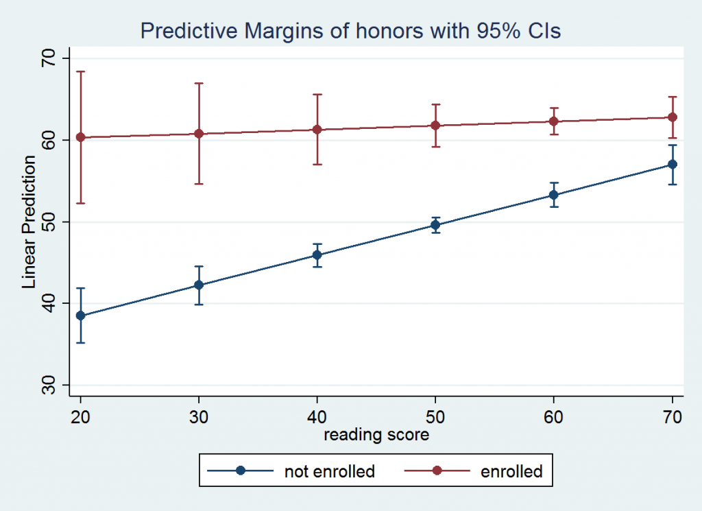
Next, we will compute the predictive margins for every 10th value from 20 through 70 of read for each level of honors. The predictive margins for this model are the linear predictions of write for the six values of read for each level of honors.
margins honors, at(read=(20(10)70)) vsquish Predictive margins Number of obs = 200 Expression : Linear prediction, predict() 1._at : read = 20 2._at : read = 30 3._at : read = 40 4._at : read = 50 5._at : read = 60 6._at : read = 70 ------------------------------------------------------------------------------ | Delta-method | Margin Std. Err. z P>|z| [95% Conf. Interval] -------------+---------------------------------------------------------------- _at#honors | 1 0 | 38.53975 1.705084 22.60 0.000 35.19785 41.88165 1 1 | 60.31129 4.090197 14.75 0.000 52.29465 68.32793 2 0 | 42.23389 1.183996 35.67 0.000 39.9133 44.55448 2 1 | 60.80504 3.121742 19.48 0.000 54.68654 66.92354 3 0 | 45.92803 .7137843 64.34 0.000 44.52904 47.32702 3 1 | 61.29879 2.177292 28.15 0.000 57.03138 65.5662 4 0 | 49.62217 .4798269 103.42 0.000 48.68172 50.56261 4 1 | 61.79254 1.309847 47.18 0.000 59.22529 64.35979 5 0 | 53.31631 .7510556 70.99 0.000 51.84427 54.78835 5 1 | 62.28629 .8188838 76.06 0.000 60.68131 63.89127 6 0 | 57.01045 1.229244 46.38 0.000 54.60117 59.41972 6 1 | 62.78004 1.26697 49.55 0.000 60.29682 65.26325 ------------------------------------------------------------------------------
Since this is a linear model, each of the six predictive margins for honors = 0 will fall on a straight line as will the six values for honors = 1. If we want to graph these values as two lines we will need the values of the predictive margins, the values of read for which the values were computed and the value of honors to which they apply. The command marginsplot will graph the output from the predictive margins.
marginsplot, x(read)
After looking at the graph you might be interested in testing whether the predictive margins for honors = 0 are different from the values for honors = 1 for each of the six values of read. If we had used the post option we could have followed up using test as a post-estimation command. However, it is easier to rerun the margins command to compute the marginal effect of honors using the dydx option. Since honors is a categorical variable margins will automatically compute the discrete change for us.
margins, dydx(honors) at(read=(20(10)70)) vsquish Average marginal effects Number of obs = 200 Expression : Linear prediction, predict() dy/dx w.r.t. : 1.honors 1._at : read = 20 2._at : read = 30 3._at : read = 40 4._at : read = 50 5._at : read = 60 6._at : read = 70 ------------------------------------------------------------------------------ | Delta-method | dy/dx Std. Err. z P>|z| [95% Conf. Interval] -------------+---------------------------------------------------------------- 1.honors | _at | 1 | 21.77154 4.364615 4.99 0.000 13.21706 30.32603 2 | 18.57115 3.298474 5.63 0.000 12.10626 25.03604 3 | 15.37076 2.276819 6.75 0.000 10.90828 19.83325 4 | 12.17037 1.400641 8.69 0.000 9.425166 14.91558 5 | 8.96998 1.101633 8.14 0.000 6.81082 11.12914 6 | 5.769589 1.714441 3.37 0.001 2.409347 9.129831 ------------------------------------------------------------------------------ Note: dy/dx for factor levels is the discrete change from the base level.
All six of these tests would be significant using a Bonferroni adjusted critical value of .05/6= .0083.
Example 2
Our next example will be a little more complex in that it has two categorical by categorical interactions (female by prog and female by honors) with one term in common between them. In addition, there is a continuous covariate, math. This time we will start with the ANOVA model and follow it with the regression model.
anova write female##prog female##honors c.math Number of obs = 200 R-squared = 0.6304 Root MSE = 5.88221 Adj R-squared = 0.6149 Source | Partial SS df MS F Prob > F --------------+---------------------------------------------------- Model | 11270.2046 8 1408.77558 40.72 0.0000 | female | 364.204296 1 364.204296 10.53 0.0014 prog | 407.481332 2 203.740666 5.89 0.0033 female#prog | 228.269898 2 114.134949 3.30 0.0390 honors | 2398.83909 1 2398.83909 69.33 0.0000 female#honors | 73.9785286 1 73.9785286 2.14 0.1453 math | 1072.64751 1 1072.64751 31.00 0.0000 | Residual | 6608.67039 191 34.6003686 --------------+---------------------------------------------------- Total | 17878.875 199 89.843593 regress write female##prog female##honors math Source | SS df MS Number of obs = 200 -------------+------------------------------ F( 8, 191) = 40.72 Model | 11270.2046 8 1408.77558 Prob > F = 0.0000 Residual | 6608.67039 191 34.6003686 R-squared = 0.6304 -------------+------------------------------ Adj R-squared = 0.6149 Total | 17878.875 199 89.843593 Root MSE = 5.8822 ------------------------------------------------------------------------------ write | Coef. Std. Err. t P>|t| [95% Conf. Interval] -------------+---------------------------------------------------------------- 1.female | 3.565842 1.786126 2.00 0.047 .0427751 7.088908 | prog | 2 | .6948486 1.613388 0.43 0.667 -2.487499 3.877196 3 | -5.665851 1.785104 -3.17 0.002 -9.186901 -2.1448 | female#prog | 1 2 | -.324647 2.152854 -0.15 0.880 -4.57107 3.921776 1 3 | 4.833603 2.425983 1.99 0.048 .0484437 9.618763 | 1.honors | 11.23618 1.710336 6.57 0.000 7.862603 14.60975 | female#| honors | 1 1 | -3.007322 2.056683 -1.46 0.145 -7.064052 1.049408 | math | .3262727 .0585993 5.57 0.000 .2106878 .4418577 _cons | 31.69696 3.168456 10.00 0.000 25.4473 37.94662 ------------------------------------------------------------------------------ testparm female#prog ( 1) 1.female#2.prog = 0 ( 2) 1.female#3.prog = 0 F( 2, 191) = 3.30 Prob > F = 0.0390 testparm i.prog ( 1) 2.prog = 0 ( 2) 3.prog = 0 F( 2, 191) = 8.35 Prob > F = 0.0003 estimates store m1
As you can see the regression and ANOVA models yield the same results for the interactions and one degree of freedom tests. The two degree of freedom test for prog is different from the anova results because regress uses indicator (dummy) coding. The testparm results for prog is actually the simple effect of prog when female is at its reference level of zero.
We will again use the margins command with the asbalanced and post options to obtain the adjusted cell means.
margins female#prog, asbalanced post Predictive margins Number of obs = 200 Expression : Linear prediction, predict() at : female (asbalanced) prog (asbalanced) honors (asbalanced) ------------------------------------------------------------------------------ | Delta-method | Margin Std. Err. z P>|z| [95% Conf. Interval] -------------+---------------------------------------------------------------- female#prog | 0 1 | 54.49168 1.445088 37.71 0.000 51.65936 57.324 0 2 | 55.18653 .9742899 56.64 0.000 53.27695 57.0961 0 3 | 48.82583 1.43898 33.93 0.000 46.00548 51.64618 1 1 | 56.55386 1.254649 45.08 0.000 54.09479 59.01292 1 2 | 56.92406 .8203316 69.39 0.000 55.31624 58.53188 1 3 | 55.72161 1.214488 45.88 0.000 53.34126 58.10196 ------------------------------------------------------------------------------
Now we can use test commands to test the simple main effects for prog at each level of female.
/* test of prog at female==0 */ test (0.female#1.prog=0.female#2.prog)(0.female#1.prog=0.female#3.prog) ( 1) 0bn.female#1bn.prog - 0bn.female#2.prog = 0 ( 2) 0bn.female#1bn.prog - 0bn.female#3.prog = 0 chi2( 2) = 16.70 Prob > chi2 = 0.0002 /* test of prog at female==1 */ test (1.female#1.prog=1.female#2.prog)(1.female#1.prog=1.female#3.prog) ( 1) 1.female#1bn.prog - 1.female#2.prog = 0 ( 2) 1.female#1bn.prog - 1.female#3.prog = 0 chi2( 2) = 0.66 Prob > chi2 = 0.7174
The critical value for these tests of simple main effects is 3.76 for a per-family error rate of .05. Thus, only the test for prog at female==0 is statistically significant. We will follow up this significant test of simple main effects with pairwise comparisons among the levels of prog.
/* pairwise comparisons for prog at female==0 */ test (0.female#1.prog=0.female#2.prog) /* prog1 vs prog2 */ ( 1) 0bn.female#1bn.prog - 0bn.female#2.prog = 0 chi2( 1) = 0.19 Prob > chi2 = 0.6667 test (0.female#1.prog=0.female#3.prog) /* prog1 vs prog3 */ ( 1) 0bn.female#1bn.prog - 0bn.female#3.prog = 0 chi2( 1) = 10.07 Prob > chi2 = 0.0015 test (0.female#2.prog=0.female#3.prog) /* prog2 vs prog3 */ ( 1) 0bn.female#2.prog - 0bn.female#3.prog = 0 chi2( 1) = 15.25 Prob > chi2 = 0.0001
The Bonferroni adjusted p-values for prog1 versus prog3 and prog2 versus prog3 are .0045 and .0003, respectively. The other pairwise comparison was not significant without any adjustment.
Next, we need to look at the second interaction in the model. To do this we will use the estimates restore command. Once the estimates are restored, we will follow the same series of steps that we used for the first interaction.
estimates restore m1 margins female#honors, asbalanced post Predictive margins Number of obs = 200 Expression : Linear prediction, predict() at : female (asbalanced) prog (asbalanced) honors (asbalanced) ------------------------------------------------------------------------------ | Delta-method | Margin Std. Err. z P>|z| [95% Conf. Interval] -------------+---------------------------------------------------------------- female#| honors | 0 0 | 47.21659 .7187761 65.69 0.000 45.80781 48.62536 0 1 | 58.45276 1.573305 37.15 0.000 55.36914 61.53639 1 0 | 52.28542 .7503273 69.68 0.000 50.8148 53.75603 1 1 | 60.51427 1.137905 53.18 0.000 58.28402 62.74452 ------------------------------------------------------------------------------ /* test of honors at female = 0 */ test 0.female#0.honors=0.female#1.honors ( 1) 0bn.female#0bn.honors - 0bn.female#1.honors = 0 chi2( 1) = 43.16 Prob > chi2 = 0.0000 /* test of honors at female = 1 */ test 1.female#0.honors=1.female#1.honors ( 1) 1.female#0bn.honors - 1.female#1.honors = 0 chi2( 1) = 35.23 Prob > chi2 = 0.0000
This time the critical value for the per family error rate is 5.10, so both tests are statistically significant.
Instead of running margins followed by test, we could have arrived at the same results by running margins with honors included in the dydx option. For categorical variables the dydx option calculates discrete change. The output for this approach is in terms of z-scores. By squaring the z-scores we can compare the results to the test command above.
estimates restore m1 margins female, dydx(honors) asbalanced post Average marginal effects Number of obs = 200 Expression : Linear prediction, predict() dy/dx w.r.t. : 1.honors at : female (asbalanced) prog (asbalanced) honors (asbalanced) ------------------------------------------------------------------------------ | Delta-method | dy/dx Std. Err. z P>|z| [95% Conf. Interval] -------------+---------------------------------------------------------------- 1.honors | female | 0 | 11.23618 1.710336 6.57 0.000 7.883979 14.58837 1 | 8.228854 1.386442 5.94 0.000 5.511478 10.94623 ------------------------------------------------------------------------------ Note: dy/dx for factor levels is the discrete change from the base level. display ([1.honors]_b[0.female]/[1.honors]_se[0.female])^2 43.159281 display ([1.honors]_b[1.female]/[1.honors]_se[1.female])^2 35.226969
Thus concludes example 2.
Source: https://stats.oarc.ucla.edu/stata/faq/how-can-i-use-the-margins-command-to-understand-multiple-interactions-in-regression-and-anova-stata-11/
0 Response to "Margins for Continuous Variable Interacted With Discrete"
Post a Comment